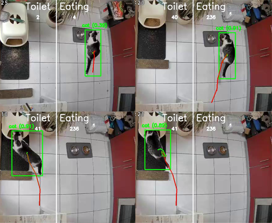
Sometimes you just need a practical scenario to dive into a new tech field. In my case, it was wanting to monitor my cat’s daily routine — when he eats and when he heads to the litter box. It wasn’t just about the curiosity of knowing his routine, but also ensuring he’s eating and doing his business as usual, which is a good indicator of a pet’s health. Also, I had a cheap webcam, I had no use for and, that was perfect for this endeavor which nudged me into the world of motion detection and object recognition, combining them to create basic yet effective pet monitoring.

All code referenced in this post, and more is available in the GitHub repository.

Object detection with YoloV8

Ultralytics, the creators of YOLOv8, made it available in 5 sizes: n, s, m, l, and x. The bigger the model, the more accurate it is, but it also requires more resources.

source: YOLOv8 Readme

Since my finished code will run in a vm on cpu only, because I do not have any ai-accelerators or gpus in my hyper visor, I have to make a tradeoff. I cannot use the x-model, even though its accuracy is fantastic. The n-model allows for a usable frame rate but is too inaccurate for my use case.
The tradeoff will be that I need to train the n-model myself to improve its accuracy for my use case.

How well each model performs on your specific device is easy to check. Take a look at this minimal viable example to detect
objects in a video using yolov8s:

Step 1: install ultralytics, numpy and opencv

open a terminal and run the following command. You can also use a virtual environment if you want to, but at least for ultralytics it makes sense to install it globally, because of its command line interface.

1

pip install ultralytics numpy opencv-python

step 2: download the model

The models are available on GitHub. You can download them for free using curl or your browser.

1

curl -L -o yolov8s.pt https://github.com/ultralytics/assets/releases/download/v0.0.0/yolov8s.pt

step 3: convert the model to onnx

We are using the *.onnx (pronounced onix) model here. This is a format optimized for even faster inference. You can convert the *.pt model to *.onnx using the following command:

1

yolo export model=yolov8s.pt format=onnx 

step 4: run the model against a video

Now we can use the model to detect objects in a video. For this, we need a video file. You can use any video file you want. I used a video of my cat eating.

1
2
3
4
5
6
7
8
9
10
11
12
13
14
15
16
17
18
19
20
21
22
23
24
25
26
27
28
29
30
31
32
33
34
35
36
37
38
39
40
41
42
43
44
45
46
47
48
49
50
51
52
53
54
55
56
57
58
59
60
61
62
63
64
65
66
67
68
69
70
71
72
73
74
75
76
77
78
79
80
81
82
83
84
85
86
87
88
89
90
91

import argparse
import cv2
import numpy as np
from ultralytics.utils import yaml_load
from ultralytics.utils.checks import check_yaml

# import class names and define colors for bounding boxes
CLASSES = yaml_load( check_yaml( 'coco128.yaml' ) )[ 'names' ]
colors = np.random.uniform( 0, 255, size = (len( CLASSES ), 3) )


# helper function that will draw the box and label for each detection
def draw_bounding_box( img, class_id, confidence, x, y, x_plus_w, y_plus_h ):
    label = f'{CLASSES[ class_id ]} ({confidence:.2f})'
    color = colors[ class_id ]
    cv2.rectangle( img, (x, y), (x_plus_w, y_plus_h), color, 2 )
    cv2.putText( img, label, (x - 10, y - 10), cv2.FONT_HERSHEY_SIMPLEX, 0.5, color, 2 )


def main( onnx_model, input_video ):
    # load model
    model = cv2.dnn.readNetFromONNX( onnx_model )
    # load video file
    cap = cv2.VideoCapture( input_video )

    # while video is opened
    while cap.isOpened( ):
        # as long as there are frames, continue
        ret, original_image = cap.read( )
        if not ret:
            break

        # the model expects the image to be 640x640
        # the following code resizes the image to 640x640 and adds black pixels to any remaining space
        [ height, width, _ ] = original_image.shape
        length = max( ( height, width ) )
        image = np.zeros( ( length, length, 3 ), np.uint8 )
        image[ 0:height, 0:width ] = original_image
        scale = length / 640
        blob = cv2.dnn.blobFromImage( image, scalefactor = 1 / 255, size = (640, 640), swapRB = True )

        # actually feed the image to the model
        model.setInput( blob )
        outputs = model.forward( )

        # the model outputs an array of results that we need to process to transform the 
        # coordinates back to the original image size, also we only want to consider detections
        # with a confidence of at least 25%
        outputs = np.array( [ cv2.transpose( outputs[ 0 ] ) ] )
        rows = outputs.shape[ 1 ]
        boxes, scores, class_ids = [ ], [ ], [ ]
        for i in range( rows ):
            classes_scores = outputs[ 0 ][ i ][ 4: ]
            ( minScore, maxScore, minClassLoc, ( x, maxClassIndex ) ) = cv2.minMaxLoc( classes_scores )
            if maxScore >= 0.25: # only consider detections with a confidence of at least 25%
                box = [
                    outputs[ 0 ][ i ][ 0 ] - ( 0.5 * outputs[ 0 ][ i ][ 2 ] ),
                    outputs[ 0 ][ i ][ 1 ] - ( 0.5 * outputs[ 0 ][ i ][ 3 ] ),
                    outputs[ 0 ][ i ][ 2 ],
                    outputs[ 0 ][ i ][ 3 ]
                ]
                boxes.append( box ), scores.append( maxScore ), class_ids.append( maxClassIndex )

        # deduplicate multiple detections of the same object in the same location
        result_boxes = cv2.dnn.NMSBoxes( boxes, scores, 0.25, 0.45, 0.5 )

        # draw the box and label for each detection into the original image
        for i in range( len( result_boxes ) ):
            index = result_boxes[ i ]
            box = boxes[ index ]
            draw_bounding_box(
                original_image, class_ids[ index ], scores[ index ],
                round( box[ 0 ] * scale ), round( box[ 1 ] * scale ),
                round( ( box[ 0 ] + box[ 2 ] ) * scale ), round( ( box[ 1 ] + box[ 3 ] ) * scale ) )
        
        # show the image
        cv2.imshow( 'video', original_image )

        if cv2.waitKey( 1 ) & 0xFF == ord( 'q' ):
            break

    cap.release( )
    cv2.destroyAllWindows( )


if __name__ == '__main__':
    parser = argparse.ArgumentParser( )
    parser.add_argument( '--model', default = 'yolov8s.onnx', help = 'Input your onnx model.' )
    parser.add_argument( '--video', default = str( './videos/video_file.mp4' ), help = 'Path to input video.' )
    args = parser.parse_args( )
    main( args.model, args.video )

Fine-tuning and training the model

Training Yolo means to create a dataset and use a the yolo train command to start the process. A training set is basically a simple folder structure with JPG-Files and corresponding TXT-Files. The TXT-Files contain the coordinates of the objects in the image. You will also need a yaml file that contains the class names and the directories that contain the training data

Step 1: create the dataset

Let’s start by creating a folder structure for our dataset. We will use the following structure:

1
2
3
4
5
6
7
8
9
10
11
12
13

-- yolo
    -- dataset
        -- images
            -- image1.jpg
            -- image2.jpg
            -- image3.jpg
                -- ...
        -- labels
            -- image1.txt
            -- image2.txt
            -- image3.txt
            -- ...
    -- training.yaml

Step 2: creating labels

The labels are simple text files that contain the coordinates of the objects in the image in the format <label_nr> <x_mid> <y_mid> <box_width> <box_height> eg.:

1

15 0.8569664001464844 0.34494996070861816 0.08885068893432617 0.40773591995239256

Creating these label files is the actual part of training your model; it takes a lot of time and effort. But the effort is worth it, because the more accurate your labels are, the better your model will be. We have basically two options to create these labels: manually or automatically.

Manually creating labels

For some images I was not able to automatically label or where the automatic labeling was not accurate enough, I created the labels manually. I used LabelImg for this. It is a simple tool that allows you to draw bounding boxes around objects in an image and save the coordinates to file. It is available for Windows, Linux and Mac. Its also rather quick to work with when using the shortcut keys.

Automatically creating labels

Since we just want to improve the accuracy of the smaller n-model, we can use the x-model to automatically label the images. This is not as accurate as manually labeling the images, but it is a good starting point.

To start, I created a 5-minute video which always contains my cat in various locations in the scene. Running that video through the n-model, I collected all the images where the model was unable to detect a cat. I then ran these images through the x-model and used the resulting labels as a starting point for my manual labeling. Using an M1 Macbook, I was able to lable most of the ~7000 frames in about 1 hour.

For some frames, even the x-model was unable to detect the cat. Also, the x-model, in a few cases, drew the bounding boxes too big so that they included parts of the background. I manually corrected these labels.

You can find the code for both of these steps in the GitHub repository for this blog post:

• detection_check.py: collects all frames where yolov8n was not able to detect a cat.
• x_check.py: runs the frames from detection_check.py through yolov8x and saves the labels to file, creating a dataset in the process.

Step 3: create the training.yaml

This is just a simple config file for the training process. Assuming your folder structure is like the one from step 1, it should look something like this:

1
2
3
4
5
6
7
8
9
10
11
12
13
14

path: ./dataset
train: images
val: images # ideally you would have a separate validation set

names:
  0: person
  1: bicycle
  2: car
  ...
  15: cat
  ...
  77: teddy bear
  78: hair drier
  79: toothbrush

see the coco128.yaml file for a complete list of all classes.

Step 4: start the training

Finally, we can start the training process. After all the preparation, this is as simple as running the following command:

1

yolo detect train data=training.yaml model=yolov8n.pt epochs=2

Explanation of the parameters:

• data: the path to the training.yaml file
• model: the model to use for training
• epochs: the number of epochs to train for, epochs are basically iterations over the entire dataset. The more epochs you train for, the more accurate your model will be. But training for too many epochs can lead to overfitting, which means that the model is too accurate for the training data and will not be able to generalize to new data. Common wisdom is to train for as many epochs as you can without overfitting. In my case, I trained for 10 epochs, which took about 12 hours on my M1 Macbook.

In the end, I used a more complex command to make use of the “hyperparameters”, which resulted in a much more confident model. This is the command I used:

1

yolo detect train data=training.yaml model=yolov8n.pt epochs=10 lr0=0.00269 lrf=0.00288 momentum=0.73375 weight_decay=0.00015 warmup_epochs=1.22935 warmup_momentum=0.1525 box=18.27875 cls=1.32899 dfl=0.56016 hsv_h=0.01148 hsv_s=0.53554 hsv_v=0.13636 degrees=0.0 translate=0.12431 scale=0.07643 shear=0.0 perspective=0.0 flipud=0.0 fliplr=0.08631 mosaic=0.42551 mixup=0.0 copy_paste=0.0

Making use of the model

Now that we have a trained model, we can use it to detect objects in images and videos. The code for this is very similar to the code we used to create the training data. You will just need to exchange the label-writing part with whatever you want to do with the detection.

In my case, I monitored an RTSP stream from my webcam using OpenCV. And each time my cat is detected, we make an entry into the database so it can we display as a Gantt-Diagram. Because the ai-model is quite cpu intensive, I also implemented motion detection to only run the model when there is motion in the scene. This is the code I used:

1
2
3
4
5
6
7
8
9
10
11
12
13
14
15
16
17
18
19
20
21
22
23
24
25
26

# OpenCV offers a background subtractor that can be used to detect motion in a scene. Depending on the history-size, 
# it has some ramp-up time until it's reliable, so the first few iterations will result in false motion detection positives
background_subtractor = cv2.createBackgroundSubtractorMOG2(history=500, varThreshold=25, detectShadows = False )

def main( onnx_model, input_video ):
    # load model
    model = cv2.dnn.readNetFromONNX( onnx_model )
    # load video file
    cap = cv2.VideoCapture( input_video )

    # while video is opened
    while cap.isOpened( ):
        # as long as there are frames, continue
        ret, original_image = cap.read( )
        if not ret:
            break

        frame_without_timestamp = original_image.copy()
        frame_without_timestamp[0:50, :] = 0  # blackout timestamp
        fgmask = background_subtractor.apply(frame_without_timestamp)

        count = cv2.countNonZero(fgmask)
        
        if count > 3750: # fine-tuned value for my use case
            # pass image to model and draw bounding boxes on detections
            # ...

full example in monitoring.py

Conclusion

Machine learning is extremely powerful and fascinating, but the surrounding math makes it intimidating and unapproachable for the uninitiated. Though, with the right tools, it is easy to get started and create something useful. I hope this blog post was helpful to you, and you will be able to create something with it. If you have any questions, feel free to reach out to me on LinkedIn or GitHub.

Browsing the web and using services often requires us to give out our email address. And in the day and age of regular data breaches, we should be careful with what we give out.
Apart, many services will hold on to your email address forever and use it for marketing purposes, even if you don’t want it, or tell them to stop.

For this use case services were invented that allow us to create a temporary email addresses, that will forward all emails to our real email address or allow us to read and answer emails in a webclient. Some are paid, some are free.
But all of them have one thing in common: They are not open source, and you have to, again, trust them with your data. Some time ago I stumbled upon this repo on GitHub. It’s a CloudFormation template that will deploy a disposable email service in your AWS account. Sadly, it’s not maintained anymore, lacks some features and relies on, as said, a CloudFormation-Template. So I decided to take the idea and build my own version of it, using the AWS-CDK.

How it works

We will utilize several AWS services to build our service. It will be all serverless. The frontend will be a static website hosted in S3, the actions triggered be the frontend will be handled by several lambda functions through an API Gateway that is protected by a Cognito User Pool.

Receiving of emails ist done by SES for which you will need to create a custom domain and verify it, before you can start this project. Two lambdas check the incoming email, and if it is for a disposable email address, we save the email to S3 and note it in a DynamoDB “Addresses”-table. The frontend will then be able to read the emails from S3. If redirect is enabled for the disposable email address, the email will be forwarded to the real email address. When doing so, we replace the original sender with a proxy address so that you can answer redirected emails directly form you email client and still keep your real email address private.

Features

• Create disposable email addresses
• send and receive attachments
• Forward emails to your real email address automatically
• Reply to forwarded emails directly from your email client and keep your real email address private
• fully fledged webclient to manage your disposable email addresses
• comprehensive wysiwyg editor to compose emails

Prerequisites

• AWS Account
• Domain that you own and can create DNS records for
  • ideally you should have a subdomain for this service, e.g. disposable.yourdomain.com
• configured SES and verified for that domain

Getting started

Install dependencies

1. If not already done you can install CDK as follows:

   1	$ npm install -g aws-cdk

2. We will also need the AWS-CLI configured to use our account. CDK will use the authentication to do all the AWS calls for us.
   Use the AWS Docs to install it, depending on your OS:
   https://docs.aws.amazon.com/cli/latest/userguide/getting-started-install.html

3. and run:

   1	$ aws configure

follow the guide and everything should be setup.

Install and deploy the project

This project consist of two repos. One for the frontend and one for the CDK which also contains the backend.

1. Clone the repos:

   1 2 3 4

   # Frontend: $ git clone https://github.com/globus243/disposable-email-frontend # Backend: $ git clone https://github.com/globus243/disposable-email-cdk

2. Install the dependencies for both repos:

   1	$ npm install

3. change the variables for the backend to fit your account and domain:

   1 2 3 4

   # edit the following files: $ disposable-email-cdk/lib/constants.ts # if your SES is not in eu-west-1, change the region in $ disposable-email-cdk/bin/disposable-email-cdk.ts

4. build the CDK project:

   1	$ npm run build

5. deploy the CDK project:

   1	$ cdk deploy

   in case of errors, try to run:

   1	$ cdk bootstrap

6. As already described, the frontend and backend are secured by a cognito user pool. The React-frontend uses an Amazon-library for authenticating with the pool, but we need to tell it which pool to use. For this we need to get the user pool id and the client id. You can find them in the AWS Console under Cognito -> User Pools -> Your Pool -> App Clients. Copy the id of the app client and the user pool id and paste them into the .env file of the frontend. Also copy the api gateway endpoint and enter the email domain.

   1	$ disposable-email-frontend/.env

7. Now we can build the frontend as well and copy the build artifacts to the StaticWebsite-directory in the CDK project:

   1 2	$ npm run build $ cp -r build/* disposable-email-cdk/src/StaticWebsite

8. finally we just deploy the thing again. don’t worry cdk is smart and skips unchanged resources:

   1	$ cdk deploy

After deployment

After the deployment is finished, you can open the frontend in your browser. Though you will find that you don’t have credentials to log in yet.
For security reasons I disabled the option of self-signup. So you will have to create a user manually. You can do so by heading back to AWS Console and going to the Cognito User Pool. Creating an Account is straight forward, so I won’t go into detail here.
When you now first login with your new account, you will be asked to change your password using a token that was sent to your email address. After that you can log in with your new password.
Also check your SES settings and verify that the correct rule set is selected. If not, select it and save the settings.

Conclusion

With this project you are now able to run your very own disposable email service. It can save you real money if you, like me, were paying for a service like this. And you can be sure that your data is safe, as you are in full control of it.
Regarding cost, most expensive part is the hosted zone which will cost around $0.6/month. But if this service is just a subdomain more for you, than the cost are negligible, and you can run it basically for free, as long as you don’t have a ton of users.
I hope you enjoyed this project. I had a lot of fun building it. If you have any questions or suggestions, feel free to contact me via GitHub.

When we monitor stuff we depend on the monitored device to be at least a bit cooperative. And while most business devices, we are used to, have no issues getting surveilled in one way or another, especially consumer devices tend to be difficult.

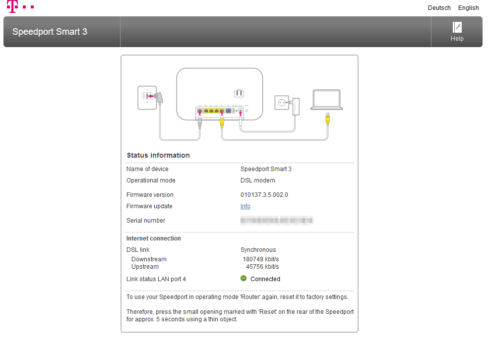
In my homelab I have such a device, a German Telekom issued Speedport Smart 3

In part 1 of this blog post we go into detail on how to monitor a Speedport Smart 3 with Nagios and in the upcoming part 2 we build an event handler to automatically react to events like low download speed.

Situation

In germany, ISPs have to provide you with a free modem when you rent an internet connection from them, the free solution for the Telekom is the Speedport. It is a fairly good device delivering most a consumer could wish for. It is not just a simple Layer 2 modem, it is also a router with DHCP, DNS, Wi-Fi, and some smart home capabilities.
But since my home lab covers all these features, I usually put these provider issued devices into modem-mode (or as close to it as possible), and connect it to my firewall which does PPPoE or what ever is needed by the provider to get a connection.

Normally that’s it, the device is dumbed down and does not respond to anything else. But the Speedport Smart 3 has a nice feature that allows one device to connect to either of Port 1-3. When this device assumes an 169.254.2.0/24 IP we can reach the Speedport under 169.254.2.1 and get a nice overview of the reported, theoretical connection speeds and also some meta information about the Speedport.

So I connected port 2 of the Speedport to a free interface of my firewall, gave the interface the appropriate IP and also, since 169.254.0.0 is a Link-local address and normally not routed by network devices, I used the proxy-feature of my firewall to make the Speedport accessible to the rest of my network.

How it works

To monitor the Speedport we have to write a custom nagios check since the data are not easily extracted from the UI the Speedport provides.
For some reason the JSON, the frontend receives from the Speedport, is encrypted. But since the password for it is also found in the frontend code, we can decrypt it but that is not something a standard check, nagios is shipped with, could do. Why it was build like this, with encrypted traffic but decryption keys in user accessible code is not known to me. I suspect an approach of security by obscurity.

Make Speedport service interfaces reachable

before nagios would be able to reach the Speedport’s service interface, we need some network magic done. I have done it two ways in the past. With routers that support routing link-local addresses you could just create a static route for 169.254.2.1 where you set the next hop to the routers interface that is connected to the speedport.

Since this has some security implications als also is not supported by my current firewall, a pfSense, I defaulted to use the integrated HA proxy feature.

Since my pfSense is virtualized, I first created a new virtual interface that terminated to a free physical interface of its host.
The pfSense interface was configured to use 169.254.2.2

I then created a front end and backend in the HA proxy settings to make the speedport reachable to my server vlan, using the pfSense IP and port 8080.

For details on how to create a working proxy configuration for HA proxy, please refer to the pfSense Docs.

Preparing Nagios

First, let us create the Nagios check. I wrote it as a python script, and it can be downloaded from this project’s GitHub repo

Copy check_speedport_connection to /opt/nagios/libexec/

make sure that your nagios host has python3 and all the requirements installed

python3 -m pip install pycryptodome requests

For installing python consult your OS’ manual.

Now we need to teach nagios how to use our new script,
In your commands.cfg, normally located at /opt/nagios/etc add:

1
2
3
4

define command {
    command_name check_speedport_connection
    command_line $USER1$/check_speedport_connection $ARG1$
}

Note: we could go really over board with defining the check here, but it’s really not necessary and also makes the syntax for using the check in the service config later on way harder.

At last, we need to actually use the check for a service.
I have for each host I monitor one file containing all its service definitions.

1
2
3
4
5
6
7
8
9
10
11
12
13
14
15
16
17
18
19
20
21
22
23
24
25
26
27
28
29
30
31
32

######### HOST DEFINITON

define host {
    host_name                Speedport 3
    use                      generic-switch
    address                  x.x.x.x 
    check_command            check_http!-H x.x.x.x -u "/html/login/modem.html" -p 8080
    max_check_attempts       2
    check_interval           5
    retry_interval           1
    check_period             24x7
    contacts                 nagiosadmin
    notification_interval    60
    notification_period      24x7
}

######### SERVICE DEFINITON

define service {
    host_name                Speedport 3
    service_description      Online state
    use                      generic-service,graphed-service
    check_command            check_speedport_connection!--hostname x.x.x.x --port 8080 --downloadWarn 178000 --downloadCrit 160000 --uploadWarn 23500 --uploadCrit 19000
    max_check_attempts       2
    ## event_handler         fix-internet ## we will be doing this in Part 2!
    check_interval           1
    retry_interval           1
    check_period             24x7
    notification_interval    60
    notification_period      24x7
    contacts                 nagiosadmin
}

Now only restarting Nagios is left either using the UI or from terminal.
After some time Nagios should start to show the state like this:

The service check also emits performance data which can be viewed by clicking the little graph symbol next to the service name.

Now You will always know when your internet speed falls below your contract’s limits. Keep in mind that this is the actual reported value from the Speedport that would also be used by Telekom support in case of disputes. By collecting e-mails or even the performance data, you have a nice source of truth.

In Part 2 we will build an event handler that is able to restart the modem using a smart home power plug. Stay tuned.

DynDNS enables us to great stuff. I use it to reach my home network on the go via a neat subdomain. Sadly, many DynDNS provider call for some kind of fee, at least if you want to use your own domain.
Good thing there is AWS, with its services Route53 and Lambda. AWS-Labs even has the working code in a GitHub repo for us but setting it up with the AWS Web Console can be tedious at best and a nightmare to maintain.

Since they posted that example much has changed in the AWS world. For example, we got the AWS CDK which makes it possible to write infrastructure as code using typescript and npm. Which in turn makes deploying stuff into AWS repeatable and easy.

So, today we are building an extensible, serverless DynDNS for your domain using CDK.

Let’s get started

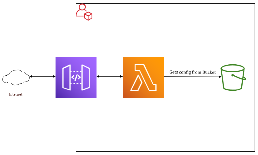
Before we start let us visualize what we are even building.
We will be using AWS ApiGateway as the internet facing component. All requests will go to the APIGateway which in turn redirects it to our Lambda.
The Lambda function will try to access the config file from the bucket and if successful it will do its magic.

How it will work

The DynDNS will be able to manage multiple zones and subdomains, depending on the configuration. For this example however, we are only making it to update one Record in a single Hosted Zone, but configuring it to do more is trivial.

The service will have two modes set and get.

The get-Mode will return the requesters IP as a json and is quite neat for all kind of programmatic applications where you have to get your external IP.
ex. https://dyndns.mydomain.com/?mode=get

The set-Mode will take 2 URL parameters hostname and hash. hostname will contain the record you are trying to update with your new IP and hash will contain, well, a hash from the combined hostname, your external IP and the shared secret.
Since the Lambda will have these values accessible inside the S3 Bucket, it can calculate the same hash we send it, and if so that means our request was “authorized” and the IP can be updated with the requesters.
ex. https://dyndns.mydomain.com/?mode=set&hostname=home.mydomain.com.&hash=d37433e52b3d945eb7cdb63c75154a62f8ebacdf4dc62fe809a341bfbe201c23

Install prerequisites

1. If not already done you can install CDK as follows:

   1	$ npm install -g aws-cdk

2. We will also need the AWS-CLI configured to use our account. CDK will use the authentication to do all the AWS calls for us.
   Use the AWS Docs to install it, depending on your OS:
   https://docs.aws.amazon.com/cli/latest/userguide/getting-started-install.html

3. and run:

   1	$ aws configure

follow the guide and everything should be setup.

Clone the repository

For convenience, I created a repo containing all the files we need.
So Only some minor changes have to be done, and we can build and deploy the package.

1

$ git clone https://github.com/globus243/AWS-DynDNS-CDK.git ./dyndns_lambda

Edit the source files

We have to change 2 things, the Domain, CDK will use to deploy the DynDNS, and the config file the Service will use during runtime.

1. On line 18 in lib/dyndns_lambda-stack.ts enter the name from the hosted zone that should be used to make the service reachable.
   So if You plan to use dyndns.mycooldomain.com you already should have a Route53 Hosted Zone called mycooldomain.com.

2. Adjust the setting to fit you: src/lambda_s3_config/config.json
   These setting will be used by the lambda during runtime to generate the hash which will have to match the hash we send on our set-request. Do not forget the trailing dot for the domain name (it is not a typo).

Deploy

When done we can actually deploy our service to AWS. It is done in 4 steps.

1. Install dependencies

   1	$ npm install

2. Translate files to js

   1	$ npm run build

3. Synthesize a cloudformation template

   1	$ cdk synth

4. deploy it to your AWS Account

   1	$ cdk deploy

And Now?

And now we have a working DynDNS service which will update our Route53 Records to the IP requesting the change, if the authorization was successful.

Go ahead and make a get-request to see if it answers:
https://dyndns.mydomain.com/?mode=get

The AWS-Lab Team has also working scripts for updating the record.
I tested this one successfully https://github.com/awslabs/route53-dynamic-dns-with-lambda/blob/master/route53-ddns-client.sh

From here on you could build a Cron job or something to call the script every x minutes to update your record.
I do this from my home automatization server.

Pricing of this solution is extremely low. Only the Hosted Zone will cost a fixed price once a year and as long as you are using it privately, you will probably never hit the free tier limits and even then, it is cents to a million requests. For me, it never made the slightest dent in my bill.